
Customer segmentation using Databricks Solution Accelerator
Wondering how to create the best marketing strategy to reach out to different customer groups? Do you know which groups of customers are most likely to buy your product? Clustering your customers into segments based on profiles, behaviours and buying patterns is the answer.
This article provides a great way jump-start your clustering project using pre-built code designed by Databricks. In earlier blogs, Get Started with Clustering: The Easy Way and 10 Incredibly Useful Clustering Algorithms You Need To Know we explained the idea of clustering through a simple example and explored the top ten clustering algorithms used by data scientists and machine learning practitioners. In this article, we will use the Databricks Solution Accelerator to perform unsupervised machine learning on a financial dataset to identify customer groups to understand customers better.
The Problem
Customer segmentation is important as it provides the ability to understand customers and their needs. This, in turn, enables targeted marketing and delivering the right message, product and service. According to a report from Ernst & Young, "A more granular understanding of consumers is no longer a nice-to-have, but a strategic and competitive imperative for banking providers. Customer understanding should be a living, breathing part of everyday business, with insights underpinning the full range of banking operations."

dataset
We will be using the German Credit dataset, a publicly available dataset provided by Dr. Hans Hofmann of the University of Hamburg. The German Credit dataset contains features describing 1000 loan applicants who have taken credit from the bank. Using this dataset, our aim will be to understand the following "How should the bank personalise its products for its customers?".
How are we going to solve this?
To perform customer segmentation, we will use the Databricks Solution Accelerators. Databricks Solution Accelerators are fully working notebooks that focus on the most frequent and high-impact use cases. The basic concept behind the accelerators is to provide their customers with pre-built code to accelerate data analytics and AI development. These notebooks are freely accessible, customisable, and can be tailored to specific use cases.
To accelerate our analysis, we will customise and tailor the Databricks customer segmentation solution accelerator to understand the loan applicants within the German Credit dataset. The customer segmentation solution accelerator is available for download using this link and consists of 4 different notebooks, each addressing different parts such as data preparation, feature engineering, clustering and profiling, respectively.
So let's start
The goal here is to investigate and utilise a dataset other than the one described in the solution accelerator to demonstrate how we can adapt the solution accelerator. As this is a different dataset to that used in the Databricks customer segmentation solution accelerator, the exploratory data analysis (EDA) and feature engineering steps are slightly different. Therefore, all steps for data preparation, EDA and feature engineering are detailed in the notebooks and can be downloaded from this link.

After importing the dataset, we carried out EDA and the summary from performing EDA analysis is as follows:
The distribution of 'Age', 'Credit_amount' and 'Duration' are skewed. We, therefore, need to apply transformations to reduce skewness and make the data a better approximation of the normal distribution. We use the log transform on 'Age', 'Credit_amount', and 'Duration', and the following plot shows the distribution before and after the transformation.

Plot showing the distribution of the features before and after the transformation
Duration and Credit amount are highly correlated as shown in the correlation plot below. This makes sense as the larger the credit amount, the longer it would take to repay the loan.
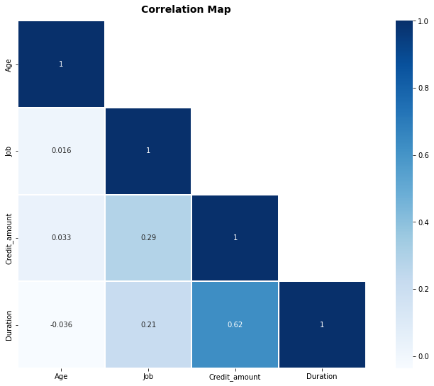
A correlation heatmap showing the correlation between the features
There are twice as many males compared to females in loan applicants.

There are 69% of male applicants and 31% of female applicants
Most applicants, about 71%, own their own home, followed by 18% rent a home.

Plot showing the distribution of loan applications owning, renting and not having a house.
A large portion of applicants requested loans for buying cars, followed by radio/TV.

Most of the loan, 33% are for purchasing cars, followed by 28% purchasing radio/TV.
The next step after the EDA is converting the categorical features into numerical features. We use label encoding to convert the categorical features into a machine-readable form, i.e., numbers.
Next, we apply use StandardScaler() to standardise and scale all the features within the dataset by subtracting the mean and then scaling to unit variance.
Before, we apply the clustering algorithm, we use Principal component analysis (PCA). PCA is a common technique used for reducing the dimensionality of datasets thus increasing interpretability but at the same time minimising information loss.
Now we are ready for clustering
Here, we use the Databricks Solution Accelerator to perform K-means clustering.
K-means is a simple, popular algorithm for dividing instances into clusters around a pre-defined number of centroids (cluster centres). The algorithm works by generating an initial set of points within the space to serve as cluster centres. Instances are then associated with the nearest of these points to form a cluster, and the true centre of the resulting cluster is re-calculated. The new centroids are then used to re-enlist cluster members. The process is repeated until a stable solution is generated (or until the maximum number of iterations is exhausted).
Demonstrate Cluster Assignment on the dataset
The challenge with K-means clustering is determining the optimal number of clusters. So, how do we do this?
We will leverage the pre-built code to help us with this.
We will calculate the sum of squared distances between members and assigned cluster centroids (inertia) to determine the optimal cluster centres. This is also known as the elbow plot and is shown below. The reason for it being termed elbow plot is due to the line plot resembling an arm, and the elbow (the point of inflection on the curve) is a good indication of the optimal number of clusters.
From the elbow plot, we can see that the total sum of squared distances between cluster members and cluster centres decreases as we increase the number of clusters in our solution. The optimal number of centres is somewhere between 3 and 4.

Elbow plot showing the point of inflection, or elbow is is somewhere between 3 and 4.
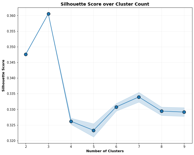
Silhouette Score over Cluster Count plot indicates that optimal clusters are 3.
As well as computing the sum of squared distances, the pre-built code in the notebook also provides the ability to compute the silhouette scores. The silhouette score provides a combined measure of inter-cluster cohesion and intra-cluster separation (ranging between -1 and 1, with higher values being better). This is another way to decide on the optimal number of clusters.
Due to the number of iterations, Databricks have also provided efficient code that uses Resilient Distributed Dataset (RDD) to distribute the work across the cluster.
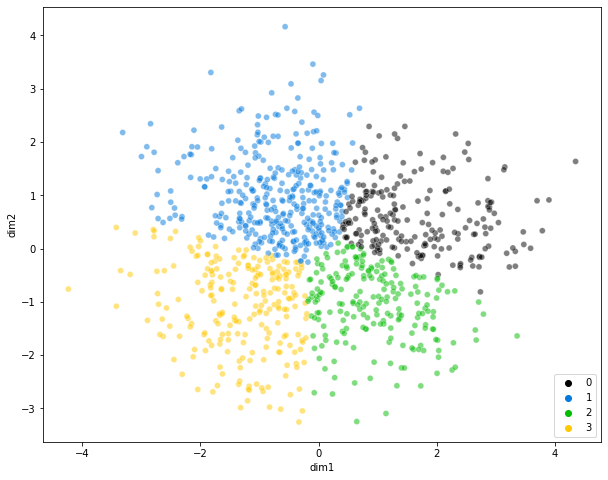
Now, we can also visualise our results to get a sense of how the clusters align with the structure of our dataset for number of clusters = 3,4 and 5.
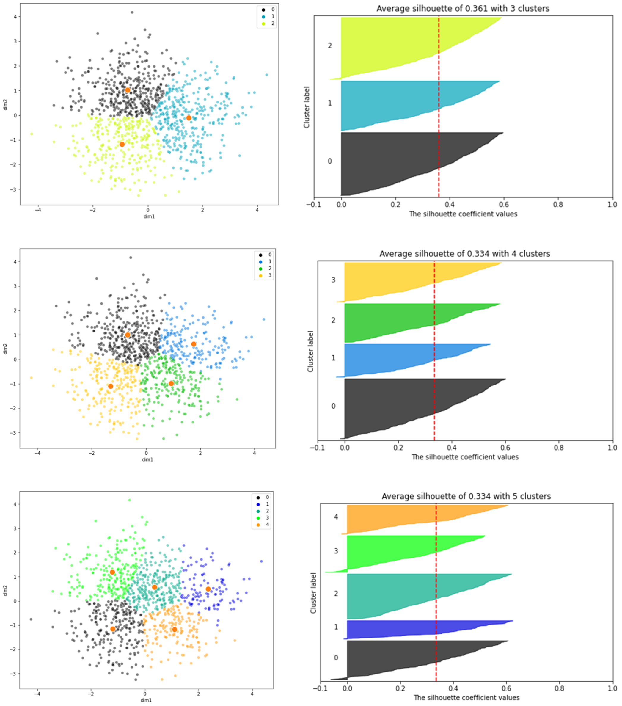
Scatter plot and Silhoutte analysis for each cluster in K-Means clustering on the dataset with clusters = 3,4 and 5
Observations from above scatter and silhouette plots:
For clusters=3, all of the plots are of comparable thickness and hence of same size, as can be considered the optimal number of clusters.
For clusters=4, although all plots have more or less the same width, the thickness varies from one cluster label to another.
The thickness of the silhouette plot for the cluster with cluster_label=1 and 4 and when clusters=5, is smaller in size.
From the plot above, we can confidently deduce that the number of optimal clusters agree with the previous elbow plot, which is 3.
What does this all mean? How can we gain insight into the segments?
The next stage is to examine how the loan applicants fit into the various groups. In our notebook, for example, we have shown how the applicants' age, job, credit amount, and length are grouped into three segments.
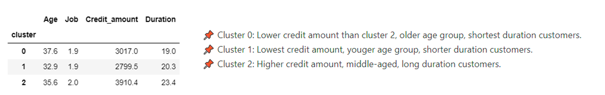
This is by no means an exhaustive analysis, and more work can certainly be directed into profiling.
That's it!
This article demonstrated the use of the Databricks Solutions Accelerator to implement K-means clustering for segmenting the loan applicants. The accelerators are fully customisable and can be adapted to other use cases with minimal tweaks. Using the K-means algorithm, we segmented the loan applicants into 3 groups which now can be used by the bank to understand the characteristics of these particular groups. This will enable the opportunity for effective targeted marketing. Another thing to try that has not been done here is to implement hierarchical clustering to the dataset to analyse the segmentation.
If you are looking at ways to segment your customer portfolio to gain insights, using the freely available Segmentation Databricks Solutions Accelerator is perfect to jump-start your machine learning project. I hope this article will provide motivation to explore the Databricks Solutions Accelerators and start using them in your machine learning use case.
If you found this helpful and want to see more of how other Databricks Solutions Accelerators are applied to different datasets, let us know by getting in touch.